Precision farming specialists say one of the first steps in moving to the variable-rate application of inputs is pinpointing the drivers of crop variation.

In a recent Society of Precision Agriculture Australia (SPAA) webinar, held with GRDC investment, three experts outlined how variable-rate cropping works and gave examples of how it can benefit grain growers.

South Australian-based Colin Hinze, a senior consultant with Pinion Advisory, said variable-rate input application was about optimising profit per hectare.

By way of example, he pointed to Figure 1, which he said could be used to represent the amount of yield variation across three paddocks.

Figure 1: Representation of soil variability across three theoretical paddocks.

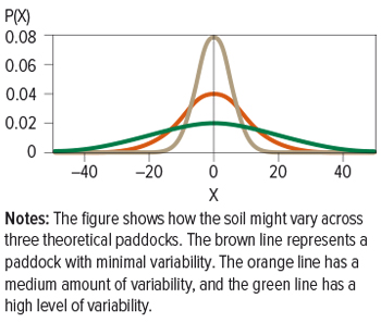
Source: Colin Hinze.

“The brown line represents a paddock with minimal variability,” Mr Hinze said.

“The orange line has a medium amount of variability, and the green line has a high level of variability.

“If the three lines depict variability in soil pH_Ca, for example, the blue line would show that pH_Ca across the paddock was similar (slightly below and above average).

“By contrast, the green line represents an area with a large range in low and high pH_Ca.

“If we take this through to a blanket management strategy for liming, there are significant areas that will be given rates that are too low and other significant areas where the rates are too high, possibly to toxic levels.

“So, this is where we might be able to apply variable-rate technology to tighten our input application around that variability.”

Mr Hinze said that precision agriculture used maps of yield, protein, biomass and soil attributes, for example, and combined these with soil testing to better understand what might be driving the variation in production.

“Once the main driver is identified, we can target inputs with variable-rate technology.

“It is a continuous improvement cycle, however, because we need to keep observing how precision-applied inputs change production over time.

“The goal is to turn a highly variable paddock into one with less variability.”

Efficiency gains

Pinion Advisory senior consultant Colin Hinze.

Optimising efficiency, he said, was about applying the right amount of the right product at the right time.

But optimising efficiency with variable-rate technology was about using the right amount of input in the right place underpinned by the right data.

When it comes to selecting the right data, Mr Hinze said, it was as simple as looking at the data you already have.

“Auto-steering systems are collecting ‘point data’ continuously that could be used to generate elevation maps,” he said.

“These could be combined with EM38 data, for example, to understand better how terrain, soil texture and soil type vary.

“Combining that data with yield maps, satellite-generated biomass data or aircraft-based biomass imagery is how you start to build a picture of potential zones in paddocks across your farm.”

The next step, he said, was checking if the data available was sufficient to address the problem you were trying to fix.

“For example, if the constraint to productivity is a soil structural issue, you would look at soil texture and type as a first step and check how that varies across the paddock,” he said.

“If the constraint is a nutritional issue, you might look at soil testing various layers in five-centimetre increments, for example, to detect a ‘hidden’ pH_Ca issue.”

Another question to ask yourself was: “Are these maps and analysis consistent with what I understand about my paddocks?”. This applies your own intuitive thinking, which is important as a test.

Other numerical tests can also be applied, for example by looking at the correlation between grain yield and soil pH_Ca.

Data layers

Mr Hinze said there were many different ways to use variable-rate technology, but exactly which data layers were used depended on the problem to be solved.

“It could be a long-term structural issue, such as water drainage, that will change a paddock’s production over time,” he said. “It might be a multi-year effect around applying lime and gypsum.

Or it could be aimed at solving issues around phosphorus and nitrogen. “The maps that you have are only as valuable as the actions they drive.

Spend time and resources on areas of the farm that you can change with actionable data.”

No 'cookie cutter'

Ag Logic director Reuben Wells.

Tasmania-based Reuben Wells, from Ag Logic, said there was no “cookie-cutter approach” to variable-rate cropping that would suit every season or grower.

By way of example, he pointed to a client from Tasmania who wanted to improve the uniformity of his ryegrass seed paddocks.

“We had a wet start to the season and saw a lot of variability in ryegrass establishment because parts of paddocks were waterlogged and other parts were dry,” Dr Wells said.

“The grower wanted to know how he could even out the maturity of his seed crop to assist harvest timing. We looked at several data sources, including biomass imagery from the Sentinel-2 satellite and drone imagery.

“We decided to use the drone imagery as our base layer because it appeared clearer than the satellite data.”

To create the prescription application maps, Dr Wells used PCT Agcloud, which was developed as a hub for various precision farming applications.

“Normally, the hub does not require the use of too much external software, but we found that we needed to do a little bit of manipulation to the drone imagery to move it into PCT Agcloud,” he said.

“I helped move the imagery into the hub, and when it was in, we left the grower to handle the rest himself.”

Dr Wells said the grower reduced the nitrogen rate on the low-vigour (red) areas to lift production and increased growth regulators on the high-vigour (blue) areas to hold development back (Figure 2) and better synchronise seed production.

Figure 2: Drone imagery (left) and prescription map (right).

Source: Reuben Wells, Ag Logic

“Follow-up satellite imagery showed his approach worked well,” he said. “The biomass production was more uniform across the paddock.”

He said the same grower was also interested in switching to variable-rate application of lime and phosphorus.

“The grower had access to elevation data and satellite imagery. He had previously used a landplane fitted with a T3RRA Cutta™ to remodel the surface of the paddock to improve water drainage.

“We looked at using a topography map and soil testing on a zone basis but decided to use grid-based soil sampling because there were a few unknowns.

Figure 3: Satellite imagery (left) and topography map (right).

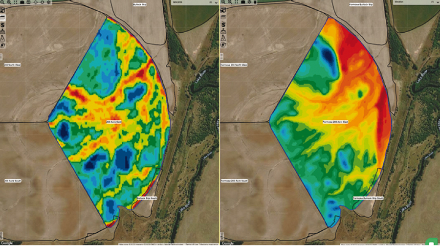
Source: Reuben Wells, Ag Logic

“Looking at biomass imagery (Figure 3) from the Sentinel-3 satellite and comparing it to a topography map, we saw a strong correlation with low vigour (red) areas and where the paddock had been waterlogged previously.

“We checked what we saw on these maps by collecting soil samples on a 0.5-hectare-sized grid basis
(Figure 4).

Figure 4: Soil sampling points (left) and surfaced pHCa map (right).

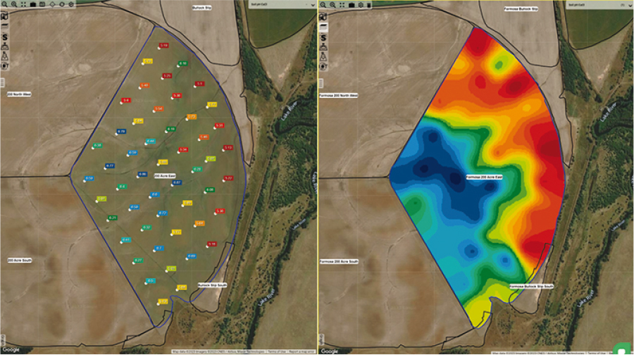
Source: Reuben Wells, Ag Logic

“In the top north side of the paddock, biomass production was high; however, pH_Ca was low or acidic.

“In the southern section of the paddock, soil pH_Ca was high or more alkaline and biomass production was high. Other parts of the paddock showed the opposite.

“We were glad we chose to gather the soil samples on a grid basis because we saw patterns that were unrelated to plant growth and topography. The variability was instead driven by paddock history.”

From there, Dr Wells said the grower set his own input rates.

“He put more lime on areas that were acidic and less lime on areas that were more alkaline. PCT Agcloud allowed the grower to link the prescription map he had created straight from the office to the tractor. The grower also created a prescription map for phosphorus, which looked similar to the pH_Ca map.

“We will continue to observe the paddock with soil tests to check how pH_Ca variability and crop production change over time.”

Zones or grids

Where possible, Dr Wells takes a zonal approach to soil testing by using biomass, yield or protein maps, if available.

“However, we have a problem in Tasmania where very little yield or protein data is available for use as a base layer.

“When you have some production zones, even if it is made from satellite biomass imagery, the benefit of a zonal soil testing system is you need to gather fewer soil samples compared with the grid-based approach.

“Deciding where the production zones will be needed requires high-quality data, or an excellent understanding of a paddock’s potential. When we don’t have that, a grid is a robust system to decide where to position soil samples.”

Prescription gypsum

Queensland-based precision agriculture specialist Tim Neale from DataFarming pointed to a client who had budgeted to apply 1.25 tonnes per hectare of gypsum across his entire farm to boost the soil sulfur supply for canola and address soil structure issues.

DataFarming director Tim Neale.

“We find most of our customers have a budget of inputs set aside, but they are unsure where it will generate the best return,” he said.

“We created some prescription maps based on last year’s biomass imagery, which is freely available to collect and use from our website.

“You just need to create an account, draw your paddocks and have a look.

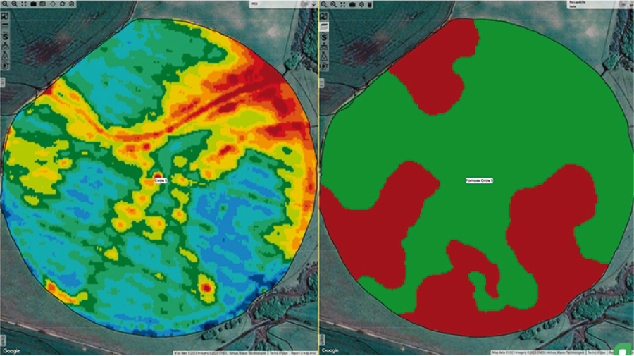
“In one grower’s case, we used September satellite imagery and divided the paddock into three zones. A light gypsum rate of 300 kilograms/ha was applied to the sandy soils – shown in Figure 5 as the blue areas – to lift the soil sulfur supply to boost canola production.

Figure 5: Grower’s variable-rate gypsum map.

Source: Tim Neale, DataFarming

“On the heavy clay – shown in red in Figure 5, where biomass production was higher – we increased the gypsum rate to  2t/ha. We used 1.25t/ha on average, but we supplied the grower with a prescription map and the total tonnes of product required for each paddock.

“It took one hour to develop the zones for 1500ha.”

Soil nitrogen bank

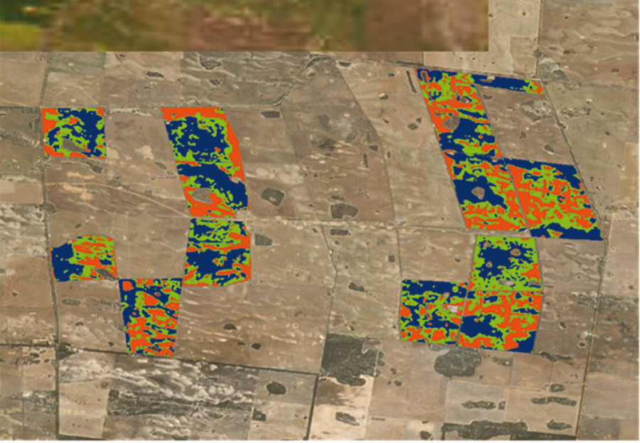
Another example, he said, involved capturing EM38 data on a client’s property on Queensland’s Darling Downs. EM38 surveys measure soil clay, water and salt, which agronomists can use to zone paddocks according to soil type.

Mr Neale then returned to the grower’s paddock to collect soil samples to assess whether there was a chemical reason for the variation in the EM38 maps.

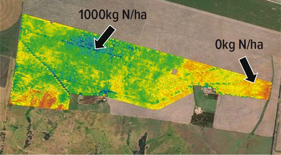
“An EM38 survey measures a depth of 1.2 metres from the soil surface,” he said. “Interestingly, we found the poorer areas had a bank of 1000kg/ha of nitrogen that had built up in the soil over 30 years (Figure 6).

Figure 6: EM38 survey.

Source: Tim Neale, DataFarming

“But the nitrogen bank was depleted in other areas down to zero available nitrogen. That’s the problem with blanket-based farming because, on average, a soil test might show 300kg/ha of nitrogen available if you collect soil samples from several parts of the field.

“But clearly, by understanding your soil type differences, you can understand the reason behind the variation.

“In this case, it was nitrogen extraction. Accordingly, a variable-rate urea map could be made based on the EM38 data, with input from soil testing, that involves converting point data into a shape file that a rate controller could read.”

Prescription urea

Mr Neale gave another example of a client who had bought a protein monitor and wanted to use the data from the device to create prescription urea maps.

“Last year, in Queensland, we had severely limited yields because of severe nitrogen deficiencies caused by flooding,” he said.

“The satellite imagery collected in September hinted at the likely final harvest yield. There was a five-fold variation in yield from 1t/ha in the red areas to 5t/ha in the blue areas (Figure 7). Coincidentally, there was a six per cent variation in protein across the field.

Figure 7: Protein to prescription urea.

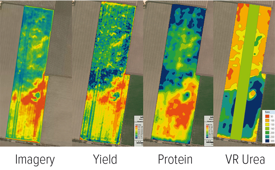
Source: Tim Neale, DataFarming

“The lowest-yielding area – shown in red in Figure 7 – had a grain protein of six per cent, and the highest yielding area – shown in blue in Figure 7 – had a grain protein of 12 per cent, demonstrating that most of the paddock was nitrogen deficient.

“We created a variable-rate prescription map based on grain protein and put a test strip through the middle to check if our approach had provided the desired results. The average rate was 160kg/ha of urea, and the urea rate varied from 50kg/ha to 300kg/ha.

“The massive yield and protein variation across the paddock is something we aim to bring under control by increasing urea rates on the low-production areas and reducing them on the higher-production areas.”

Starter fertiliser

In another example, Mr Neale worked with a grower to carry out an EM38 survey to determine the soil type differences based on clay, salt and moisture content.

Figure 8: Site-specific starter fertiliser.

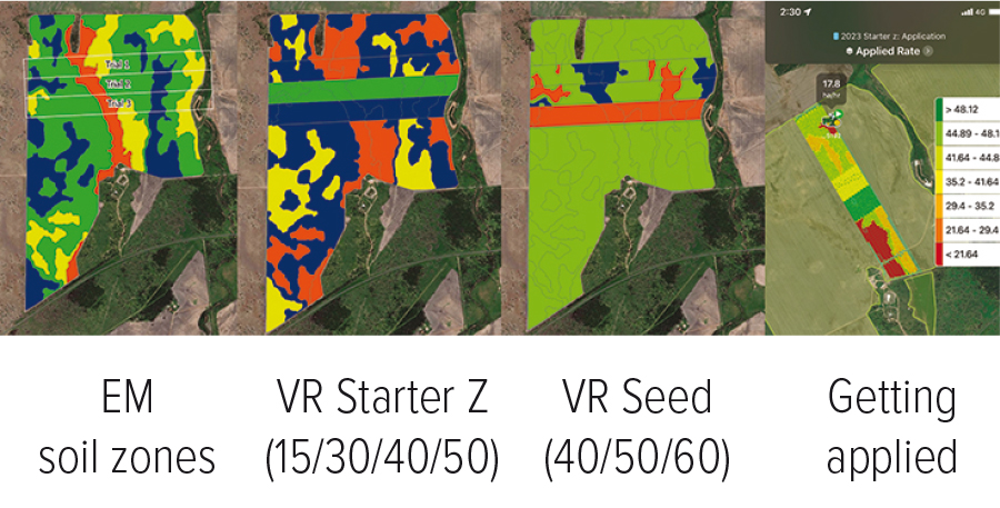
Source: Tim Neale, DataFarming

He said the red areas shown in Figure 8 equated to light soil, while the blue areas equated to heavier country.

“The grower’s agronomist collected soil samples from each area and discovered phosphorus availability was correlated with the soil type map created from the EM38 survey.

“The lighter country was lower in plant-available phosphorus, while the heavier country was higher in plant-available phosphorus.

“We produced a prescription map for starter fertiliser with monoammonium phosphate (MAP) rates at 15kg/ha, 30kg/ha and 40kg/ha based on zone-based soil sampling.

“We ran trials through the middle of the paddock to check the accuracy of our approach.

“The grower farms his country in a north-south direction, so we made the trial strips 150m wide to ensure the yield data collected was sufficient to assess our approach.

“We also set up a trial based on plant density by testing sowing rates of 40kg/ha, 50kg/ha and 60kg/ha to explore whether we need to increase the seeding rate on the lighter soils.

“Variable-rate technology makes establishing on-farm trials easy. We can assess the approach’s merits when we source the yield data after harvest.”

Simplicity important

Mr Neale said precision farming systems built in the past had been designed for use by specialised agronomists.

“Unless we can simplify precision agriculture considerably, we are not going to achieve adoption of the technology,” he said.

“Our company is on a journey to make precision agriculture automated, or semi-automated, as much as possible.

“This means using simple layers to produce simple prescription maps so people can start on a variable-rate application journey. Yield data is the ultimate measure of variability, but often that’s unavailable, so biomass imagery is a close second.”

Mr Neale said a common mistake people made when putting in test strips was inadvertently establishing them in the best part of the paddock, which often resulted in a nil response.

“You’ll often see a better response if you test the product on a poor part of the paddock,” he explained.

“Start with some understanding of the paddock – whether that’s via a yield map, farmer knowledge, a satellite image or multiple years of biomass imagery – and put in your test strips to cover the low, medium and high-productivity areas.”

Putting it together

GRDC grower relations manager – north, Graeme Sandral, said some of the key considerations for applying variable-rate technology included the following.

1. The magnitude of variability: Does the paddock have large variation for an important trait such as plant establishment, dry matter, grain yield or grain protein that can be addressed to improve overall profitability?
2. The distribution of the variation: Is the variation highly dispersed and sporadic across the paddock, or is it clustered into larger areas that are manageable with variable rate applicators?
3. Type of variation: Spatial variation refers to both across the paddock (horizontal) and through the soil profile (vertical), while temporal refers to the consistency of the variation from year to year and crop to crop.
4. The primary cause of the variability: Dispersive sodic soil at depth may not be cost-effective to address. However, significant variations in nitrogen, phosphorus, soil pH_Ca or surface dispersive sodicity can be addressed with adequate attention to detail.
5. Correlation does not always equal causality: Take care when using indirect measures of variability, as sometimes the relationship with the trait under consideration can have a low correlation. For example, measuring soil nitrogen on a grid basis is expensive. Some indirect measures can include EM38, NDVI and grain protein. However, these traits can be affected by other factors unrelated to nitrogen. This is where professional assistance can be particularly helpful in developing a deeper understanding. Accordingly, paddock strips can be used to confirm or reject the use of an indirect measure.
6. Always remember that the goal is to improve long-term profitability by maximising the returns on inputs.

More information: Colin Hinze, chinze@pinionadvisory.com; Reuben Wells, reuben@aglogic.com.au; Tim Neale, tim@datafarming.com.au

Read also: SPAA fact sheets.

Watch: SPAA GRDC Variable Rate Technology Webinar.