The ability to zone paddocks relative to susceptibility to heat and frost damage is under development using data-driven modelling to help growers better manage climate constraints

Heat stress is estimated to cost the Australian grains industry $1.1 billion every year, with frost damage accounting for a further $360 million. For both these stresses, opportunities exist to apply analytics to map and estimate the yield lost, which in turn allows growers to zone, plan and manage within-field variability in winter grains.

In 2022, GRDC invested in the development of heat and frost management analytics through a project headed by the University of Sydney Precision Agriculture Laboratory in a collaboration with Precision Cropping Technologies (PCT) Agcloud.

The project exploits historical yield monitor data and publicly available spatial maps of weather, satellite imagery, soil and landscapes. This data-driven approach makes use of machine-learning models to predict the spatial distribution of frost and heat occurrence. Since the spatial maps have national coverage, the opportunity exists to scale this from neighbouring farms to grain-growing subregions.

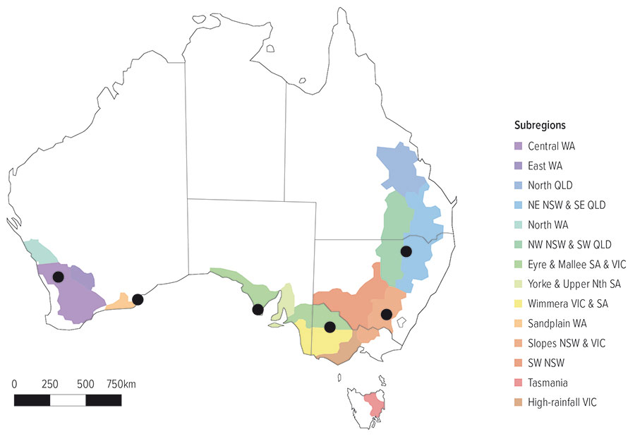
To highlight the benefit of this approach, a case study provides an overview of some preliminary work in frost identification across six groups of farms (see Figure 1) covering about 59,000 hectares. Many of these farms have yield data dating back to 2014. The study area will expand as the project progresses and also include heat stress.

Figure 1: Approximate locations of case study farms (black dots).

Source: The University of Sydney

Case study

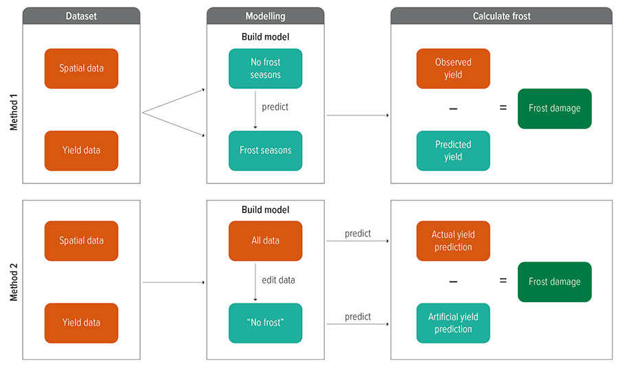
Two methods to derive frost maps are at proof-of-concept stage, with Figure 2 highlighting the difference between these methods.

Method 1 involves building local or farm-specific models using yield data from seasons that do not experience severe frost.

When this model is used to make predictions with seasonal data that experienced frost, the model predicts yield as if there had not been a frost event.

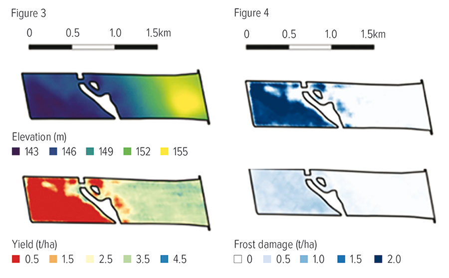
The difference between the predicted and the observed yield is then used to identify the location and severity of frost. This can be displayed as a frost damage map (see the top map in Figure 4).

Method 2 builds a model with all yield data available, as well as variables that could indicate frost (such as the number of days with a minimum temperature below 2°C). The model is applied to the original data to obtain an ‘actual yield’ prediction that should reflect the impact of frost.

Figure 2: A diagram of two data-driven methods to derive frost maps from yield monitor data and publicly available spatial datasets.

Source: The University of Sydney

The frost variables in the original data are then altered to mimic the same field with no frost. For example, a field that experiences five days with a minimum temperature below 2°C is altered to zero days. When the model is applied to the edited data, the model sees no frost events and gives an ‘artificial yield’ prediction. This is a similar concept to a space-for-time substitution used in other disciplines such as soil science.

The difference between the actual and artificial yield predictions again returns a frost damage map.

Figure 3 shows an example of a  frost-affected paddock. The frost damage maps (derived by each method) for that same paddock are shown in Figure 4.

In the example provided, the lowest yielding areas in the field are the lower-lying areas due to the accumulation of cooler air (Figure 3). Both frost maps in Figure 4 capture the spatial pattern of frost damage; however, it is difficult to quantify the actual yield lost, given it cannot be measured.

Figure 3: An example of a frost-impacted wheat field from Western Australia in 2016 (bottom) and the respective elevation map (top);
Figure 4: Frost damage maps for the same landscape as shown in Figure 3 derived using Method 1 (top) and Method 2 (bottom).

Source: The University of Sydney

Next steps

The main limitation to this approach is that no model or yield prediction is perfect. There is bound to be some degree of error.

Over the next year, the aim is to improve the accuracy of the underlying yield models and frost maps and apply similar approaches to quantify heat stress. A robust yield model means predictions could be transferable beyond the farms in the training data to other farms in the same area.

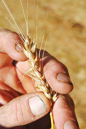Close-up photo of frost-damaged wheat. Photo: Natalie Lee

A constraint with the dataset is the low spatial resolution of publicly available daily temperature grids, the finest resolution being ANUCLIM at 1.5 kilometres. This is still too coarse to identify frost events within a field solely from temperature.

CSIRO is leading another project that is spatially downscaling land surface temperature collected by Himawari 8 (2k spatial resolution, 10-minute revisit) to acquire finer-resolution spatial datasets.

Collaboration with growers and agronomists to record past and upcoming frost events at the within-field level is ongoing. This data will be used to validate the frost damage maps in terms of location and magnitude.

The team is keen to work with any growers or agronomists who are interested in being a part of the project.

Once the method is developed and proven, it will be deployed by PCT on its Agcloud platform.

Work is underway to develop a pre-sowing tool to help growers manage frost risk and a post-frost tool to estimate yield lost in-season.  

More information: Patrick Filippi, patrick.filippi@sydney.edu.au; Si Yang Han, siyang.han@sydney.edu.au