Key points

• Crop responses to soil amelioration can differ wildly, even in paddocks with similar soil constraints
• Finding where to apply ameliorants for maximum gain can be challenging
• There is no crop model that can accommodate changes in soil chemistry or structure to simulate crop yield response from amelioration for a specific soil
• A spatial amelioration expert has created a method to better guide soil investment decisions

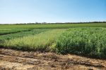
Within the same paddock, soils often have similar constraints and require the same amelioration application rates. Yet, crop responses to that amelioration can differ wildly.

It makes finding exactly where to apply ameliorants for maximum gain challenging, says spatial amelioration expert Dr Stirling Roberton.

Formerly at the University of Southern Queensland (USQ) and now at CSIRO, Dr Roberton says crop responses to amelioration are complex, non-linear and soil specific. The method, detailed below, was developed to help soil and precision agriculture specialists with amelioration investment decisions.

“These investments can be substantial, and we want to move the paradigm from annual investments to capital ones,” he says.

When making these investments, we want to be confident that they are only being applied to areas of the paddock where they are needed, and there is some indication of what the likely return on investment (ROI) will be before expenditure is made.

Dr Roberton says there is no crop model that can accommodate changes in soil chemistry or structure to simulate crop yield response from amelioration for a specific soil.

With that in mind, six regional core soil amelioration trials were established – from Forbes in New South Wales’ central west to Westmar in Queensland’s Western Downs.

“They are invaluable in providing a broad indication of what crop responses are achievable, but are limited. This is because soil constraints and their severity are highly spatially variable.

“Within a single paddock, a variety of soil amelioration strategies may be considered, all on a variable-rate basis. And even if we get the diagnosis correct, there is still no indication of what the likely ROI may be.

“Are you better off investing in areas of the paddock that require six tonnes per hectare of gypsum, or the areas that only require 2t/ha? Which will provide the best return? Which soils should you invest in?”

These investments can be substantial, and we want to move the paradigm from annual investments to capital ones.

Dr Roberton says this prompted the new method developed with GRDC support during his time at USQ.

GRDC’s John Rochecouste looked after the project within the northern Soils, Nutrition, Agronomy and Farming Systems portfolio, now called Sustainable Cropping Systems and led by Dr Cristina Martinez.

Mr Rochecouste says the method developed will help soil and precision agriculture specialists to make important investment calculations.

In turn, growers can use those calculations to make business plans. “These investments are significant and should be treated as such, with known payback periods, for example.”

The strip trial sites are now being looked after by the University of New England under ongoing GRDC investment.

Dr Roberton has taken on a new role as a research scientist at CSIRO, working on the Australian National Soil Information System (ANSIS) project. CSIRO is leading the $15 million project to redevelop Australia’s national soil information infrastructure to provide mechanisms to access and federate soil data and information through a collaborative partnership.

John Rochecouste is now Manager, Sustainable Cropping Systems – North at GRDC.

The method

Step 1 – Initial sampling

This step seeks to broadly identify the main constraints and their spatial variability across the paddock. Electromagnetic imaging (EMI) data, elevation data, yield data, gamma radiometric data, long-term normalised difference vegetation index (NDVI) information and grower experience can be drawn on to identify four sampling locations.

Step 2 – Constraint diagnosis

The second step requires diagnosing soil constraints from the four extracted soil cores at multiple depths through the profile: zero to 10 centimetres, 10 to 20cm, 40 to 50cm and 60 to 70cm for each soil core. The analysis is done in the laboratory and includes soil pH, soil EC, exchangeable sodium percentage (ESP), texture, aggregate stability, bulk density and nutrient analysis.

Dr Stirling Roberton says the sample size is not sufficient to accurately diagnose the extent of constraints or design variable-rate management plans. “It merely provides an indication of the range of issues the grower is dealing with and helps when considering amelioration strategies.”

Step 3 – Trial design, implementation and benchmark sampling

Once constraints have been diagnosed, treatments are designed according to the most-severe constraint. The treatments are placed where the constraint is, and in other spots, to pick up on constraints’ spatial variability.

Dr Roberton says that, in this approach, there will be areas where treatment is both over-applied and under-applied. “The only way to avoid this is to increase sampling density to design a variable-rate trial plan prior to implementation. While this is possible, a more cost-effective initial solution is to initially blanket-apply the treatment strip, and then back-calculate where over-application and under-application was achieved.”

A key component of the methodology is the intensive benchmark soil sampling, taken along each treatment strip. “These samples are used in the latter steps to identify which soil constraint types are providing the largest yield response.”

Step 4 – Observe and map yield response

Over several seasons, yield data should be collected and analysed across the trial site.

Dr Roberton says this should involve a yield response calculation. This is where every harvested point along each strip is compared directly to its closest control point in the nil strip.

“Undertaking this style of spatial analysis identifies which parts of the strip are contributing the biggest yield responses.”

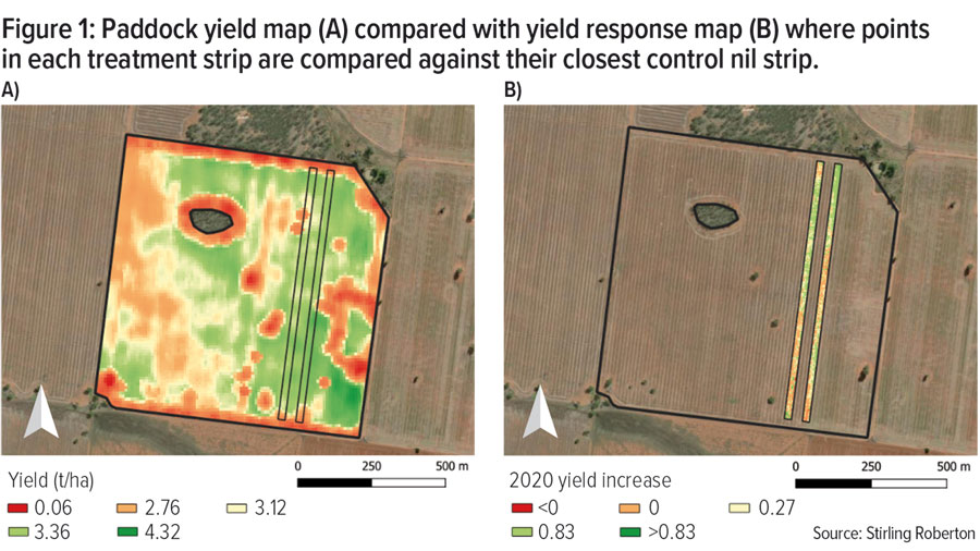
Figure 1 is an example of this type of analysis.

“When only observing the entire yield map in Figure 1B, no visual responses in the treatment strips can be observed. However, after undertaking spatial analysis of the strips and comparing each point to its closest control point, it is apparent that there are areas of each strip contributing about 0.8t/ha yield increase, which may be considered significant.

“These soil constraints or types may represent a larger area across the paddock. Using this approach, it is possible to identify which soils offer the greatest potential to benefit from soil amelioration.”

Step 5 – Paddock and farm analysis

The final step, he says, extrapolates yield responses to estimate which other areas are likely to produce a similar yield response if amelioration was attempted.

This requires two sub-steps. The first is looking at the benchmark soil samples’ laboratory analysis, and the second an intensive soil survey across the remainder of the paddock or farm to map soil constraints at a fine scale.

Dr Roberton concedes that although mapping soil constraints will require increased investment in soil sampling, the dataset will be valuable in identifying where the largest yield responses are – if amelioration is attempted.

“This sampling investment may be considered as a due diligence step prior to making a substantial soil amelioration investment.”

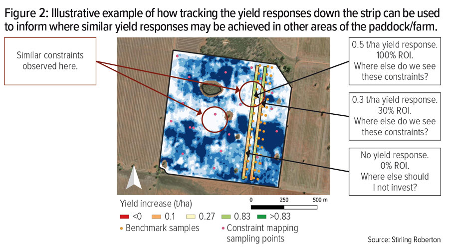
Figure 2 provides an example of how the yield responses obtained from the treatment strips can be coupled with paddock maps to identify areas that are likely to provide a similar response.

More information: Stirling Roberton, stirling.roberton@csiro.au